Tradeoff Simplicity-Accuracy

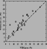
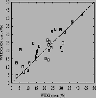
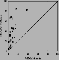
Experiments were carried out using three variants of WIDC: with optimistic pruning (o), with pessimistic pruning (p), and without pruning ($\emptyset$). Table 1 presents some results on various datasets, most of which were taken from the UCI repository of machine learning database [Blake et al.1998]. For each dataset, the eventual discretization of attributes was performed following previous recommendations and experimental setups [de Carvalho Gomes Gascuel1994]. The results were computed using a ten-fold stratified cross validation procedure [Quinlan1996]. The least errors for WIDC are underlined for each domain. For the sake of comparisons, column ``Others'' points out various results for other algorithms, intended to help getting a general picture of what can be the performances of efficient approaches with different outputs (decision lists, trees, committees, etc.), in terms of errors (and, when applicable, sizes). Some of the most relevant results for WIDC are summarized in the scatterplots of Table 2.

Table 1: Experimental results using WIDC.

	WIDC(o)			WIDC(p)			WIDC($\emptyset$)
Domain	err$\%$	$r_{DC}$	$l_{DC}$	err$\%$	$r_{DC}$	$l_{DC}$	err$\%$	$r_{DC}$	$l_{DC}$	Other
Australian	$\underline{15.57}$	$1.1$	$1.8$	$16.00$	$1.6$	$4.1$	$18.14$	$4.8$	$17.5$	$15.1_{39.0}$ f
Balance	$22.38$	$4.1$	$10.5$	$14.76$	$9.9$	$27.3$	$\underline{14.29}$	$18.7$	$44.9$	$20.1_{86.0}$ f
Breast-W	$7.46$	$1.1$	$4.5$	$\underline{4.08}$	$5.0$	$21.0$	$6.90$	$7.7$	$29.3$	$4.9_{21.8}$ f
Bupa	$\underline{36.57}$	$3.2$	$12.4$	$37.14$	$4.3$	$16.6$	$37.14$	$7.7$	$28.4$	$37.3_{37.0}$ f
Echo	$32.14$	$1.8$	$3.9$	$\underline{27.86}$	$4.7$	$11.1$	$31.42$	$24.6$	$38.8$	$32.3_{35.4}$ a
Glass2	$21.76$	$1.5$	$4.7$	$\underline{21.17}$	$1.7$	$5.4$	$26.47$	$4.3$	$12.5$	$26.3_{8.0}$ f
Heart-S	$24.07$	$3.1$	$8.9$	$\underline{19.48}$	$8.5$	$31.4$	$21.85$	$12.5$	$40.8$	$21.5$ c
Heart-C	$22.90$	$2.9$	$9.1$	$\underline{21.85}$	$6.5$	$27.4$	$25.48$	$13.3$	$46.2$	$22.5_{52.0}$ a
Heart-H	$22.67$	$3.9$	$10.9$	$20.45$	$8.4$	$24.2$	$\underline{20.00}$	$14.3$	$43.5$	$21.8_{60.3}$ a
Hepatitis	$20.59$	$3.4$	$8.7$	$19.24$	$7.0$	$17.0$	$\underline{15.29}$	$11.4$	$26.7$	$19.2_{34.0}$ a
Horse	$\underline{15.26}$	$1.7$	$3.6$	$15.57$	$3.8$	$10.4$	$20.26$	$12.5$	$31.7$	$15.7_{13.4}$ f
Iris	$\underline{5.33}$	$1.9$	$4.6$	$\underline{5.33}$	$2.9$	$7.1$	$20.67$	$3.7$	$7.9$	$8.5$ c
Labor	$\underline{15.00}$	$2.9$	$5.0$	$\underline{15.00}$	$3.7$	$6.6$	$16.67$	$3.8$	$6.7$	$16.31_{6.8}$ d
LED7	$31.09$	$6.9$	$8.4$	$24.82$	$16.2$	$21.3$	$\underline{24.73}$	$19.0$	$25.4$	$25.73_{12.2}$ d
LEDeven	$13.17$	$2.7$	$6.1$	$\underline{12.43}$	$3.8$	$9.2$	$24.63$	$9.9$	$21.9$	$13.00_{19.2}$ f
LEDeven2	$30.00$	$4.1$	$16.4$	$23.15$	$7.1$	$26.1$	$\underline{21.70}$	$24.4$	$83.8$	$23.1_{25.4}$ f
Lung	$\underline{42.50}$	$1.3$	$3.8$	$\underline{42.50}$	$2.6$	$7.1$	$\underline{42.50}$	$2.7$	$7.2$	$46.6$ e
Monk1	$\underline{15.00}$	$4.1$	$9.5$	$\underline{15.00}$	$5.2$	$13.0$	$\underline{15.00}$	$9.4$	$17.9$	$16.66_{5.0}$ d
Monk2	$24.43$	$9.0$	$38.4$	$\underline{21.48}$	$18.2$	$61.3$	$31.80$	$24.8$	$82.1$	$29.39_{18.0}$ d
Monk3	$\underline{3.04}$	$3.6$	$4.8$	$9.89$	$4.7$	$8.9$	$12.50$	$9.3$	$12.3$	$2.67_{2.0}$ d
Pima	$29.61$	$2.2$	$5.9$	$\underline{26.17}$	$8.0$	$29.4$	$32.99$	$22.2$	$68.9$	$25.9$ c
Pole	$36.67$	$1.5$	$4.1$	$\underline{33.52}$	$4.2$	$12.7$	$37.64$	$24.0$	$65.8$	$35.5_{81.6}$ f
Shuttle	$\underline{3.27}$	$1.0$	$2.0$	$\underline{3.27}$	$1.0$	$2.0$	$4.51$	$2.0$	$4.0$	$1.7_{29.8}$ f
TicTacToe	$22.47$	$5.7$	$14.4$	$\underline{20.10}$	$6.7$	$17.6$	$23.50$	$15.9$	$43.7$	$18.3_{130.9}$ f
Vehicle2	$\underline{26.47}$	$2.8$	$7.8$	$26.70$	$4.0$	$11.2$	$33.18$	$16.4$	$46.5$	$25.6_{43.0}$ f
Vote0	$\underline{6.81}$	$1.9$	$3.0$	$8.40$	$4.5$	$8.5$	$10.00$	$9.5$	$18.9$	$4.3_{49.6}$ a
Vote1	$10.90$	$2.0$	$3.5$	$\underline{9.98}$	$7.0$	$14.9$	$12.50$	$13.6$	$29.7$	$10.89_{6.4}$ d
Waveform	$30.49$	$4.8$	$8.2$	$23.47$	$7.5$	$17.3$	$\underline{20.24}$	$40.1$	$65.0$	$33.5_{21.8}$ b
Wine	$10.00$	$3.0$	$6.2$	$9.47$	$3.7$	$8.1$	$\underline{7.89}$	$4.2$	$8.9$	$22.8$ e
XD6	$\underline{16.73}$	$5.2$	$14.4$	$17.50$	$6.2$	$17.1$	$22.69$	$19.8$	$52.0$	$21.2_{58.0}$ f

Conventions: $l_{DC}$ is the whole number of literals of a DC, $r_{DC}$ is its number of rules. For ``Others'', numbers are given on the form $\mbox{error}_{(\mbox{size})}$, where a is improved CN2 (CN2-POE) building DLs, size is the number of literals [Domingos1998]. b is ICDL building DLs, notations follow a [Nock Jappy1998]. c is C4.5 [Franck Witten1998]. d is IDC building DCs, notations follow a [Nock Gascuel1995]. e is 1-Nearest Neighbor rule and f is C4.5 (pruned, default parameters) building DTs; the size of a tree is its whole number of nodes.

Table 2: Scatterplots summarizing some results of Table 1 for the three flavors of WIDC, in terms of error (first row) and size ($l_{DC}$, second row), on the thirty datasets. Each point above the $x=y$ line depicts a dataset for which the algorithm in abscissa performs better.

The interpretation of Table 1 using only errors gives the advantage to WIDC with pessimistic pruning, all the more as WIDC(p) has the advantage of providing simpler formulas than WIDC($\emptyset$), and has a much simpler pruning stage than WIDC(o). Results also compare favorably to the ``Other'' results, building either DLs, DTs, or DCs. They are all the more interesting if we compare the errors in the light of the sizes obtained. For the ``Echo'' domain, WIDC with pessimistic pruning beats improved CN2 by two points, but the DC obtained contains roughly eight times fewer literals than CN2-POE's decision list. If we except ``Vote0'', on all other problems on which we dispose of CN2-POE's results, we outperform CN2-POE on both accuracy and size. Finally, on ``Vote0'', note that WIDC with optimistic pruning is slightly outperformed by CN2-POE by $2.51\%$, but the DC obtained is fifteen times smaller than the decision list of CN2-POE. If we dwell on the results of C4.5, similar conclusions can be brought: on 12 out of 13 datasets on which we ran C4.5, WIDC(p) finds smaller formulas, and still beats C4.5's accuracy on 9 of them. A quantitative comparison of $l_{DC}$ against the number of nodes of the DTs shows that on 4 datasets out of the 13 (Pole, Shuttle, TicTacToe, Australian), the DCs are more than 6 times smaller, while they only incur a loss in accuracy for 2 of them, and limited to 1.8$\%$. For this latter problem (TicTacToe), a glimpse at Table 1 shows that the DCs, with less than 7 rules on average, keeps comparatively most of the information contained in DTs having more than a hundred leaves. On many problems where mining issues are crucial, such a size reduction would be well worth the (comparatively slight) loss in accuracy, because we keep a significant part of the information on very small classifiers, thus likely to be interpretable.