

Next: AUC Calculation
Up: Experiments
Previous: Datasets
A ROC curve for SMOTE is produced by using C4.5 or Ripper to create a classifier for each one of a series of
modified training datasets. A given ROC curve is produced by first over-sampling the minority class to a specified
degree and then under-sampling the
majority class at increasing degrees to generate the successive points on the curve. The amount of
under-sampling is identical to plain under-sampling. So, each corresponding point on each ROC curve
for a dataset represents the same number of majority class samples. Different ROC curves are
produced by starting with different levels of minority over-sampling. ROC curves were also
generated by varying the loss ratio in Ripper from 0.9 to 0.001 and by varying the priors of the
minority class from the original distribution to up to 50 times the majority class for a Naive
Bayes Classifier.
Table 2:
Dataset distribution
| Dataset |
Majority Class |
Minority Class |
| Pima |
500 |
268 |
| Phoneme |
3818 |
1586 |
| Adult |
37155 |
11687 |
| E-state |
46869 |
6351 |
| Satimage |
5809 |
626 |
| Forest Cover |
35754 |
2747 |
| Oil |
896 |
41 |
| Mammography |
10923 |
260 |
| Can |
435512 |
8360 |
Figures 9 through 23 show the experimental ROC curves obtained
for the nine datasets with the three classifiers. The ROC curve for plain
under-sampling of the majority class [19,18,17,1] is compared with our approach of
combining synthetic minority class over-sampling (SMOTE) with majority class under-sampling. The plain
under-sampling curve is labeled ``Under'', and the SMOTE and under-sampling combination ROC curve is
labeled ``SMOTE''. Depending on the size and relative imbalance of the dataset, one to five SMOTE and
under-sampling curves are created. We only show the best results from SMOTE combined with under-sampling
and the plain under-sampling curve in the graphs. The SMOTE ROC curve from C4.5 is also compared
with the ROC curve obtained from varying the priors of minority class using a Naive Bayes
classifier -- labeled as ``Naive Bayes''. ``SMOTE'', ``Under'', and
``Loss Ratio'' ROC curves, generated
using Ripper are also compared. For a given family of ROC curves, an ROC convex
hull [1] is generated. The ROC convex hull is generated using the Graham's algorithm
[35].
For reference, we show the ROC curve that would be obtained using minority over-sampling by replication in
Figure 19.
Figure 7:
Phoneme. Comparison of SMOTE-C4.5, Under-C4.5, and Naive Bayes.
SMOTE-C4.5 dominates over Naive Bayes and Under-C4.5 in the ROC space. SMOTE-C4.5 classifiers
are potentially optimal classifiers.
 |
Figure 8:
Phoneme. Comparison of SMOTE-Ripper, Under-Ripper, and modifying Loss Ratio in Ripper. SMOTE-Ripper dominates
over Under-Ripper and Loss Ratio in the ROC space. More SMOTE-Ripper classifiers lie on the ROC convex hull.
 |
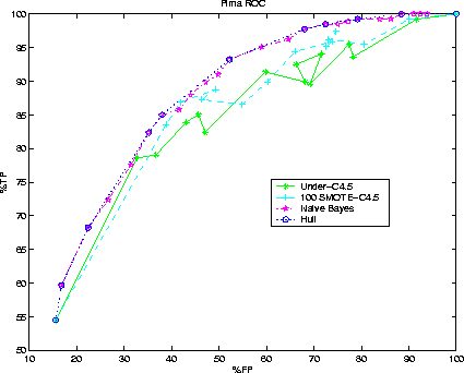
Figure 9:
Pima Indians Diabetes. Comparison of SMOTE-C4.5, Under-C4.5, and Naive Bayes.
Naive Bayes dominates over SMOTE-C4.5 in the ROC space.
 |
Figure 10:
Pima Indians Diabetes. Comparison of SMOTE-Ripper, Under-Ripper, and modifying Loss Ratio in Ripper.
SMOTE-Ripper dominates over Under-Ripper and Loss Ratio in the ROC space.
 |
Each point on the ROC curve is the result of either a classifier (C4.5 or Ripper) learned for a particular combination
of under-sampling and SMOTE, a classifier (C4.5 or Ripper) learned with plain under-sampling, or a classifier (Ripper)
learned using some loss ratio or a classifier (Naive Bayes) learned for a different prior for the minority class. Each
point represents the average (%TP and %FP) 10-fold cross-validation result. The lower leftmost point for a given ROC
curve is from the raw dataset, without any majority class under-sampling or minority class over-sampling. The minority
class was over-sampled at 50%, 100%, 200%, 300%, 400%, 500%. The majority class was under-sampled at 10%, 15%,
25%, 50%, 75%, 100%, 125%, 150%, 175%, 200%, 300%, 400%, 500%, 600%, 700%, 800%, 1000%, and 2000%. The
amount of majority class under-sampling and minority class over-sampling depended on the dataset size and class
proportions. For instance, consider the ROC curves in Figure 17 for the mammography dataset. There are three
curves -- one for plain majority class under-sampling in which the range of under-sampling is varied between 5%
and 2000% at different intervals, one for a combination of SMOTE and majority class under-sampling, and one for Naive
Bayes -- and one ROC convex hull curve. The ROC curve shown in Figure 17 is for the minority class
over-sampled at 400%. Each point on the SMOTE ROC curves represents a combination of (synthetic) over-sampling and
under-sampling, the amount of under-sampling follows the same range as for plain under-sampling. For a better
understanding of the ROC graphs, we have shown different sets of ROC curves for one of our datasets in Appendix A.
Figure 11:
Satimage. Comparison of SMOTE-C4.5, Under-C4.5, and Naive Bayes. The ROC curves of Naive Bayes and
SMOTE-C4.5 show an overlap; however, at higher TP's more points from SMOTE-C4.5 lie on the
ROC convex hull.
 |
Figure 12:
Satimage. Comparison of SMOTE-Ripper, Under-Ripper, and modifying Loss Ratio in Ripper. SMOTE-Ripper dominates the ROC space.
The ROC convex hull is mostly
constructed with points from SMOTE-Ripper.
 |
For the Can dataset, we had to SMOTE to a lesser degree than for
the other datasets due to the structural nature of the dataset. For the
Can dataset there is a structural neighborhood already established in the
mesh geometry, so SMOTE can lead to creating neighbors which are under the
surface (and hence not interesting), since we are looking at the feature
space of physics variables and not the structural information.
The ROC curves show a trend that as we increase the amount of under-sampling coupled with
over-sampling, our minority classification accuracy increases, of course at the expense of more
majority class errors. For almost all the ROC curves, the SMOTE approach dominates. Adhering to the
definition of ROC convex hull, most of the potentially optimal classifiers are the ones generated
with SMOTE.
Figure 13:
Forest Cover. Comparison of SMOTE-C4.5, Under-C4.5, and Naive Bayes. SMOTE-C4.5 and Under-C4.5 ROC curves are very close to each other. However, more points from the SMOTE-C4.5 ROC curve lie on the ROC convex hull, thus establishing a dominance.
 |
Figure 14:
Forest Cover. Comparison of SMOTE-Ripper, Under-Ripper, and modifying Loss Ratio in Ripper. SMOTE-Ripper shows a
domination in the ROC space. More points from SMOTE-Ripper curve lie on the ROC convex hull.
 |
Figure 15:
Oil. Comparison of SMOTE-C4.5, Under-C4.5, and Naive Bayes. Although, SMOTE-C4.5 and Under-C4.5 ROC curves intersect at points, more points from SMOTE-C4.5 curve lie on the ROC convex hull.
 |
Figure 16:
Oil. Comparison of SMOTE-Ripper, Under-Ripper, and modifying Loss Ratio in Ripper. Under-Ripper and
SMOTE-Ripper curves intersect, and more points from the Under-Ripper curve lie on the ROC convex hull.
 |
Figure 17:
Mammography. Comparison of
SMOTE-C4.5, Under-C4.5, and Naive Bayes. SMOTE-C4.5 and Under-C4.5 curves intersect in the ROC space; however, by
virtue of number of points on the ROC convex hull, SMOTE-C4.5 has more potentially optimal classifiers.
 |
Figure 18:
Mammography. Comparison of SMOTE-Ripper, Under-Ripper, and modifying Loss Ratio in Ripper. SMOTE-Ripper
dominates the ROC space for TP > 75%.
 |
Figure 19:
A comparison of over-sampling minority class examples by SMOTE and over-sampling the
minority class examples by replication for the Mammography dataset.
 |
Figure 20:
E-state. (a) Comparison of SMOTE-C4.5, Under-C4.5, and Naive Bayes. SMOTE-C4.5 and Under-C4.5 curves
intersect in the ROC space; however, SMOTE-C4.5 has more
potentially optimal classifiers, based on the number of points on the ROC convex hull.
 |
Figure 21:
E-state. Comparison of SMOTE-Ripper, Under-Ripper, and modifying Loss Ratio in Ripper. SMOTE-Ripper has more
potentially optimal classifiers, based on the number of points on the ROC convex hull.
 |
Figure 22:
Can. Comparison of SMOTE-C4.5, Under-C4.5, and Naive Bayes. SMOTE-C4.5 and Under-C4.5 ROC curves overlap for
most of the ROC space.
 |
Figure 23:
Can. Comparison of SMOTE-Ripper,
Under-Ripper, and modifying Loss Ratio in Ripper. SMOTE-Ripper and Under-Ripper ROC curves overlap for most of the ROC
space.
 |


Next: AUC Calculation
Up: Experiments
Previous: Datasets
Nitesh Chawla (CS)
6/2/2002


