
What is locally weighted regression?
Locally weighted regression links.
Examples of locally weighted linear regression.
Educational implementation of locally weighted linear regression.

What is locally weighted regression?
Locally weighted polynomial regression is a form of instance-based (a.k.a. memory-based) algorithm for learning continuous non-linear mappings from real-valued input vectors to real-valued output vectors. It is particularly appropriate for learning complex highly non-linear functions of up to about 30 inputs from noisy data. Both classical and Bayesian linear regression analysis tools can be extended to work in the locally weighted framework, providing confidence intervals on predictions, on gradient estimates and on noise estimates. For a full derivation and in depth discussion of locally weighted regression, see the first paper in the next section of this document.

Locally weighted regression links.

Examples of locally weighted linear regression.
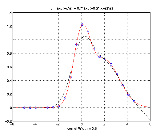
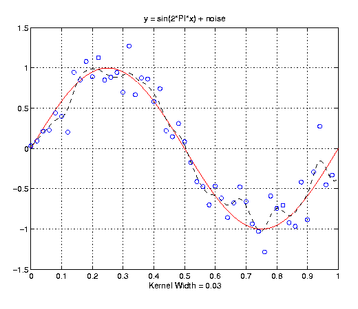
The following graphs show two examples of locally weighted linear regression. In these graphs, the blue circles show the training points, the red line shows the true function, and the dashed black line shows the regressed function. The code and datasets used to generate the points for these graphs are given in the next section of this document.
The first example is the sum of two gaussians. Specifically, y = exp(-x^2) + 0.7*exp(-0.3*(x-2)^2). In the first graph, the kernel width equals 0.15 and gives an excellent fit to the training points. In the second graph, the kernel width equals 0.8 and still gives a pretty good fit to the training points, but loses some of the details of the function.


The next example is a noisy sin curve: y = sin(2*PI*x) + noise, where noise is a guassian random variable with mean 0 and standard deviation 0.2. In the first graph, the kernel width equals 0.1 and gives a very nice fit the the training points. In the second graph, the kernel width equals 0.03 and is overfitting the data.


Educational implementation of locally weighted linear regression.
lwpr.c is an unsophisticated, stand-alone implementation of locally weighted linear regression. It can be compiled with the following command: gcc lwpr.c -lm -o lwpr. To run the program, execute the command:
lwpr <datafile> <testfile> <kwidth>
where datafile contains the training set, testfile contains the test
set, and kwidth is the kernel width. Each row of the datafile should
contain exactly the number of input dimensions + 1 numbers, separated
by spaces. The testfile should have the same format. It is important
not to place any blank lines at the beginning of the files, or any stray
characters throughout the files.
The program will use points in the datafile to predict the output for each point in the testfile and print the predicted and actual outputs. It will also print the root mean square error of the predicted outputs. The training and test sets used in the examples above are gauss.train, gauss.test , sin.train, and sin.test.
lwpr.c can be easily modified to implement higher order polynomials (or any other set of basis functions, for that matter). Because the code does not scale the input variables, the proper kernel width may be several orders of magnitude larger or smaller than the ones shown in the examples above. If you find that many of the predicted outputs are near 0 when they should not be, this generally indicates that the kernel width is far too small.