Overview
Prepare
Images
Each input image is split into
its three channels by cutting the overall image in thirds from the top down.
The margins of each channel image are then removed, 10% cropped from each side,
to make modified images on which alignment is performed. This removes the
border areas that are not part of the real image; the borders can confuse the
alignment metric as they are different on each channel. It doesn’t matter if
some of the image is removed in this step as there will be plenty of
information remaining to perform the alignment and the un-cropped images can be
used later for the final combined color image. In
fact the amount of cropping can be increased further to speed up image
alignment, by reducing the total number of pixels to be considered, as long as
there is some interesting stuff in the center of the
image.
Alignment
The green and red channels are
separately aligned with the blue channel returning optimal offsets relative to
the blue channel. This alignment is done by trying a range of offsets, in 2
dimensions, of the green or red image from the blue image and calculating an
alignment score. The score is only calculated over the overlapping portion of
each image for a given offset. The alignment score can be a number of metrics,
in this case the ‘sum of square differences’ (ssd) is
used. The ssd is calculated by first taking the
difference between the intensities of each pixel in the overlapping portions,
squaring the differences, summing over all the pixels and normalizing with the
number of pixels. The normalization is required because the overlapping region
can change size depending on the amount of offset. The ssd
basically tells us the average difference between the two images being aligned, therefore we want this score to be minimized. The
alignment that returns the lowest score is returned as the optimal alignment
offset.
Naive
Implementation
In the naive implementation,
used on the small jpeg images, the channels are directly compared for
alignment. This requires that a large region of offsets is considered, in this
case ±15 pixels in both directions, to ensure the optimal offset is found.
While fine for small images this would take a prohibitively large amount of
time on the large images.
Multi-Level
Implementation
In the multi-level implementation we
first build an image pyramid for each color channel.
This means the original image is stored at a number of different scales, each
one half the size of the previous. The shrinking can be done by convolving with
a Gaussian then sub-sampling every second pixel, in
this case imresize in Matlab
was used. Once we have the pyramid the alignment operation is first performed
on the smallest scale image and the resulting offset used as the starting point
for alignment on the next size up. The process is repeated all the way down the
pyramid until we have the optimal offset for the original image. This allows
the region of offsets we consider at each level to be much smaller, in this
case ±2 pixels, as we have an approximate guess from the previous level and at
the smallest level ±2 pixels is a significant portion of the image. This is
most significant at the larger levels where there are lots of pixels to
consider when calculating the alignment score. Overall this method is much
faster than the naive implementation on large images.
Display
The un-cropped green and red
channel images are shifted by the offsets calculated during image alignment and
combined with the un-cropped blue channel image to construct an aligned color image.
Small Image Results – Naive Method
Click images to download full-size file

File: 00088v.jpg
Offset: Green [3, 3], Red [4,5]

File 00106v.jpg
Offset: Green [4,1], Red[9,-1]

File: 00137v.jpg
Offset: Green [6,6], Red [11,8]

File: 00757v.jpg
Offset: Green [2,3], Red [5,5]

File: 00888v.jpg
Offset: Green [6,1], Red [12,0]

File: 00889v.jpg
Offset: Green [2,2], Red [4,3]

File: 00907v.jpg
Offset: Green [3,1], Red[6,0]

File: 00911v.jpg
Offset: Green [1,-1], Red [13,-1]

File: 01031v.jpg
Offset: Green [1,1], Red [4,2]

File: 01880v.jpg
Offset: Green [6,2], Red [14,4]
Large Image Results – Multi-Level Method
Click images to download full-size file

File: 00029u.tif
Offset: Green [39,16], Red [91,34]

File: 00087u.tif
Offset: Green [48,38], Red [108,55]

File: 00128u.tif
Offset: Green [35,25], Red [52,38]

File: 00737u.tif
Offset: Green [15,7], Red [49,14]

File: 00822u.tif
Offset: Green [57,25], Red [125,33]

File: 00892u.tif
Offset: Green [16,2], Red [43,2]

File: 00992u.tif
Offset: Green [50,13], Red [113,19]
File: 01043u.tif
Offset: Green [-16,10], Red [11,17]
File: 01085u.tif
Offset: Green [43,32], Red [111,59]

File: 01734u.tif
Offset: Green [48,29], Red [101,49]
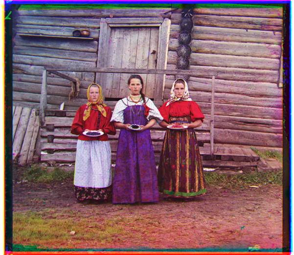
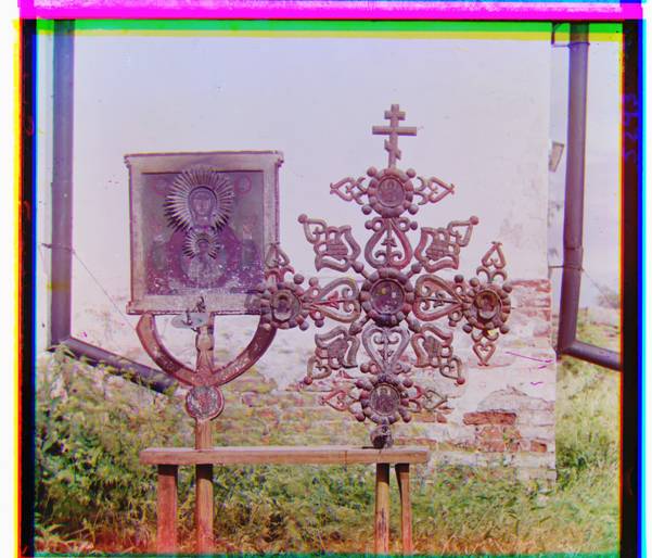
Extra Images – Multi-Level Method
Click images to download full-size file

File: 00118u.tif
Offset: Green [41,23], Red [114,21]

File: 00458u.tif
Offset: Green [42,6], Red [87,32]