Introduction

The purpose of this project was to create an algorithm that from the Gorskii photo collection negatives (an example of such a negative) will create color pictures with the best possible alignment of the channels. As some of the negatives had relatively high resolution (~60MB .tiff files) we also had to use Gaussian pyramids so that the algorithm will be able to scale easily.

Approach

Given the picture, by splitting it into three equal parts we get the three channels R, G, B. We try to match R and B and G and B separately and then we combine the results. The matching is done by moving the other channel within a specified window of translations while keeping B fixed. But applying this directly didn't work with only this picture because the channels have border effects. The simple solution that worked very well was to just remove 10% of each side of the picture. Then, using some heuristics we trim the borders of the picture where we have some strange colors as a result of the format of the original plate. Finally, some contrast adjustments are made to make the picture look more realistic.

Distance Measure

I have tried both the Eucledian metric and the Normalized Cross-Correlation (NCC), but applying them directly on the images did not produce satisfying results because the channels themselves have different intensities. To overcome this problem, I have instead tried to minimize the difference of the numerical gradients (as computed by MATLAB's gradient). Or more precisely, if A and B are the gradients of the pictures I tried to minimize n(|A-B|) where n is the sum of all the entries in the argument matrix and |X| represents the matrix obtained by taking absolute values of the entries of X (i.e. |X|[i,j] = norm(X[i,j])).

Gaussian Pyramids

To be able to handle large resolutions when two channels X and Y were aligned, first their Gaussian pyramids were created in an incremental way until we get a level of sufficient size (around 300-400 pixels). Then the matching was performed in an incremental way from the coarsest level to finer levels, improving our estimate on the way and of course reducing the size of the window of translations.

Removing Border Effects

As already mentioned, because of the nature of the negative plates the results from the previous phase had some strange colors. These borders contained black and white regions and also some very intense random colors. The algorithm that was employed used two heuristics when removing these borders, namely

Lines that were completely black or white (within a small specified error interval) were discarded.
For every line, the average of the absolute values of the normalized correlations between the three channels was computed. If this value was under a specified constant, then the line was discarded.

As an example, the pictures below show the difference after this method was applied (using a slightly higher threshold than the one for the pictures presented in the Results section).

Setting the parameter too high produced almost-perfect results for some pictures, but some were cropped too much. On the other hand, setting it too low worked for some pictures but some still had think boundary. To show the variaton on the algorithm on the pictures, all the pictures below have been processed using the same fine-tuned constants unless otherwise stated in the box below the picture.

Picture Enhancement

I have tried several enhancement techniques, including the popular white balancing (using the Gray World enhancement) and histogram equalization. But, these did not give naturally looking results. I used a different technique, namely the gray levels were remapped to use the whole interval using MATLAB's imadjust. Some results of this procedure are shown below.

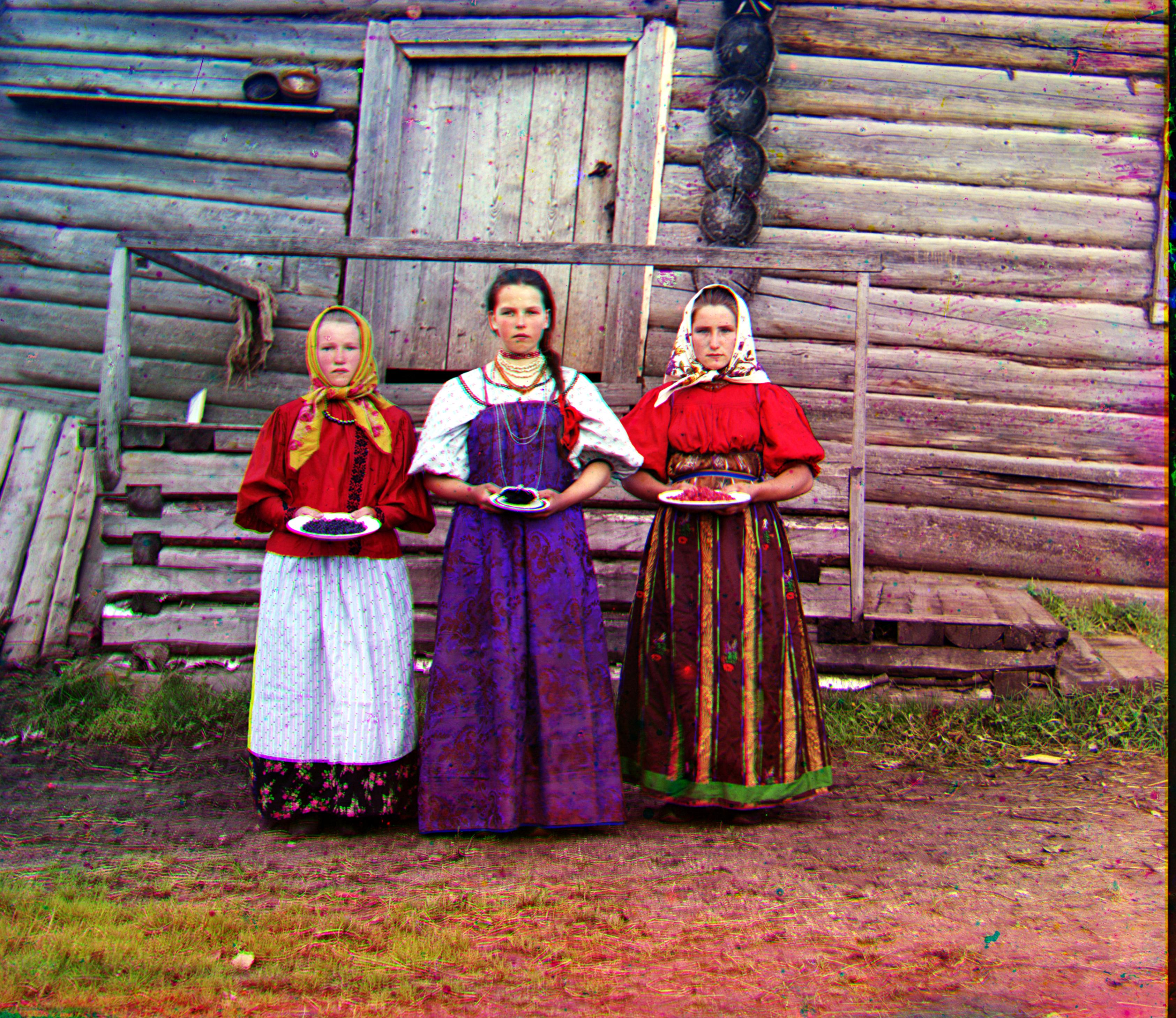
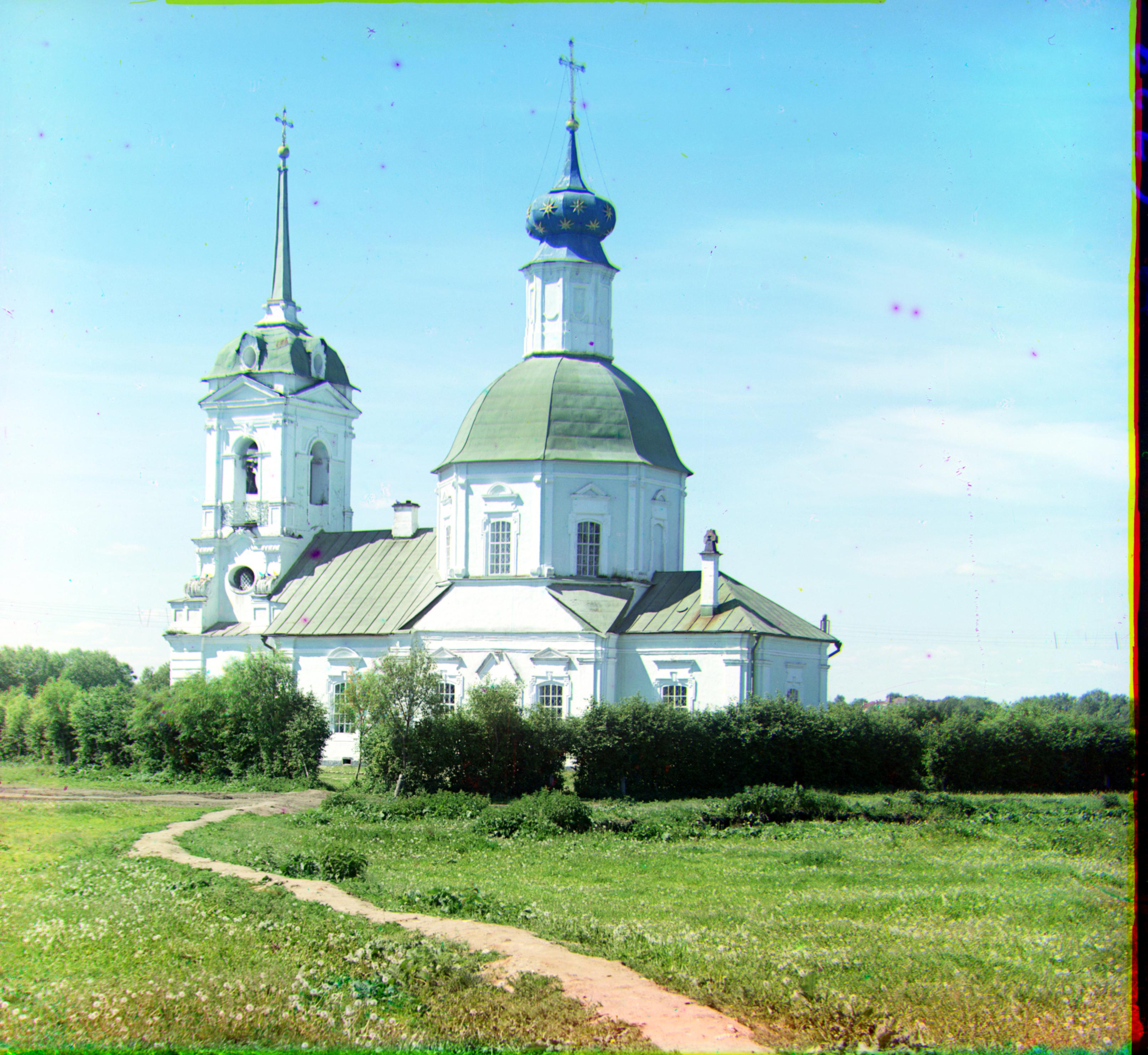
Results

The results below were obtained by running the algorithm on the provided samples and as well on other pictures from the Gorskii photo collection. The constants that were used were as follows

The error interval for black/white lines was set to 0.05
The lower bound on the correlation was set to 0.315

Together with every picture, the name of the original file is given and the displacements of the red and the green channel. The first component is displacement in the y-direction (up/down) and the second component is in the x-direction (left/right). Note that every picture after it was matched it was also cropped and the contrast has been enhanced using the techniques presented above.

Low Resolution Pictures

These were generated using the match_img function directly with a window of size 15x15.

For the first picture (00125v.jpg) the threshold on correlation was lowered to 0.19, as the cropping algorithm took too much of the border.

Provided Pictures


Image Name: `00125v.jpg` Red Displacement: `[10 1]` Green Displacement: `[5 2]`	Image Name: `00149v.jpg` Red Displacement: `[9 2]` Green Displacement: `[4 2]`	Image Name: `00153v.jpg` Red Displacement: `[14 4]` Green Displacement: `[7 3]`

Image Name: `00163v.jpg` Red Displacement: `[-4 1]` Green Displacement: `[-3 1]`	Image Name: `00351v.jpg` Red Displacement: `[13 1]` Green Displacement: `[4 1]`	Image Name: `00398v.jpg` Red Displacement: `[11 4]` Green Displacement: `[5 3]`

Image Name: `00564v.jpg` Red Displacement: `[11 0]` Green Displacement: `[5 0]`	Image Name: `00640v.jpg` Red Displacement: `[9 0]` Green Displacement: `[2 0]`	Image Name: `01112v.jpg` Red Displacement: `[5 1]` Green Displacement: `[0 0]`

Image Name: `31421v.jpg` Red Displacement: `[13 0]` Green Displacement: `[8 0]`

Pictures of my Choice


Image Name: `01210v.jpg` Red Displacement: `[15 0]` Green Displacement: `[7 1]`	Image Name: `00403v.jpg` Red Displacement: `[13 -1]` Green Displacement: `[7 0]`	Image Name: `00541v.jpg` Red Displacement: `[7 -4]` Green Displacement: `[3 -3]`

Image Name: `01106v.jpg` Red Displacement: `[13 4]` Green Displacement: `[6 3]`	Image Name: `01239v.jpg` Red Displacement: `[15 -1]` Green Displacement: `[8 0]`	Image Name: `01478v.jpg` Red Displacement: `[10 0]` Green Displacement: `[1 0]`

Image Name: `01479v.jpg` Red Displacement: `[15 0]` Green Displacement: `[4 1]`

High Resolution Pictures

For the following pictures the approach using Gaussian pyramids was used. The window size linearly decreased as we went down the pyramid. I.e. at level i a square window with side i was used (the level with highest resolution was 1). To be able to navigate the pictures more easily, a smaller version than the original is provided here. If you want to see the original version, click on the picture (they have been converted to jpeg because of web space constraints).

Provided Images

Image Name: 00458u.jpg
Red Displacement: [85 29]
Green Displacement: [41 7]

Image Name: 00911u.jpg
Red Displacement: [133 -12]
Green Displacement: [13 5]

Image Name: 01043u.jpg
Red Displacement: [12 15]
Green Displacement: [-17 10]

This picture was generated with a smaller threshold for cropping, 0.18

Image Name: 01047u.jpg
Red Displacement: [71 33]
Green Displacement: [25 19]

Image Name: 01194u.jpg
Red Displacement: [106 60]
Green Displacement: [50 39]

Image Name: 01657u.jpg
Red Displacement: [120 13]
Green Displacement: [56 9]

Image Name: 01861a.jpg
Red Displacement: [147 62]
Green Displacement: [71 39]

Pictures of my Choice

Image Name: 01427u.jpg
Red Displacement: [140 47]
Green Displacement: [67 24]

Image Name: 01779u.jpg
Red Displacement: [115 28]
Green Displacement: [51 21]

Image Name: 00882a.jpg
Red Displacement: [107 -55]
Green Displacement: [53 -23]

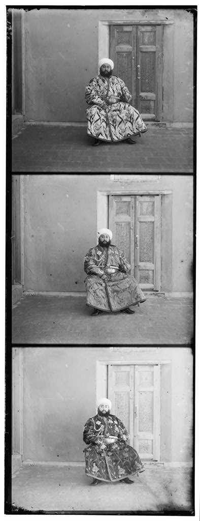
A Small Experiment of Mine

With my camera I took three pictures one after another with a bit of displacement between them. Then from each of them I extracted a different color channel and stacked them vertically. These is the result.