15-862 Computational Photography
Introduction
The algorithm implemented to colorize the photographs of Sergei Prokudin-Gorskii for this project may be broadly divided into three phases:
1. Color Channel Alignment: The algorithm first determines the offset vectors necessary to translate the green and red layers of Prokudin-Gorskii's images into alignment with the blue layer. For "small" images, this is done via a brute-force search over a window of [-20, 20] in each direction; the correctness of the alignment is judged by examining the Normalized Cross-Correlation between the channels at each offset. For "large" images (i.e. > 800px wide), a "multiscale pyramid"/"coarse-to-fine" approach is used (implemented via recursion). The image is repeatedly resized by a factor of 0.5 until it is ~400px across, then the brute-force search is applied as in the base case. This calculated offset is then used as an estimate and is refined at each level as the recursive calls return through progressively larger images. (These "refinements" require a much smaller search window (typically [-2,2] or less), dramatically improving performance).
2. Automatic Cropping: The algorithm next attempts to improve the appearance of the colorized images by several techniques, the first of which is automatic border cropping. It may be observed that the edges of Prokudin-Gorskii images often fall into the following two categories:
- Color Edges: Side-effects from the alignment, where one or more color channels are missing from a given edge. Shows abnormally large variation between the values of the R, G, and B channels.
- Black or White Borders: From Prokudin-Gorskii's negative, or the Library of Congress scanning thereof. Shows abnormally low or high brightness compared to other parts of the image.
The cropping algorithm calculates the standard deviation between the R, G, and B channels at each pixel, and also their mean. It next finds the mean of these measures across each row and down each column. The algorithm scans inward from each of the four edges of the image and crops away those rows or columns which are deemed "too far away" from the overall mean (brightness) or standard deviation (variation between color channels) of the image as a whole.
3. Automatic Color & Contrast: The discussion in lecture regarding the HSV color space inspires the algorithm's final phase: automatic color and contrast adjustment. As we lack detailed information about Prokudin-Gorskii's camera, it is somewhat difficult to suggest reasonable enhancements to the (H)ue information. While various approaches could be used (e.g. the "Gray World Assumption," or attempting to identify a white point in the image), many Prokudin-Gorskii images already have "reasonable" white balance. Therefore, these techniques often result in adjustments that are either too small to be worthwhile, or are extreme to the point of ridiculousness.
The Prokudin-Gorskii images do, however, often appear "faded" or "washed-out" compared to modern photographs. We can change this by converting to the HSV color space, making alterations to the (S)aturation and (V)alue channels, and then converting back to RGB. In both cases, the general approach is to identify "low" and "high" threshold points of the S and V values currently in the image, then apply a mathematical operation to "stretch" this input range to a wider range at the output. The expansion of the (S)aturation channel results in a wider range of colors (from subtle, nearly gray shades to extremely vivid, bright ones), while the expansion of the (V)alue channel increases contrast in the traditional sense. (To reduce the appearance of artificially "overdone" color and contrast, neither adjustment outputs the full [0,1] range of these parameters).
The overall effect of the automatic enhancements described above may be seen in the following comparison, taken from one of the assigned images:
 |
 |
Results (Assigned Images)
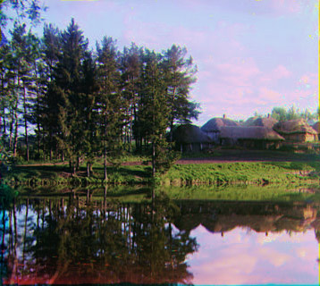
Below are results for the assigned images which I consider to be entirely successful. Each of these images was aligned, cropped, and adjusted for color and contrast entirely within Matlab and without any user intervention beyond providing the input and output filename; only the JPEG encoding and resizing for web presentation were accomplished elsewhere (specifically via Adobe Photoshop CS3). Each image is accompanied by the alignment vectors used for the green and red layers, the automatically-calculated cropping rectangle, and data on saturation and brightness. On the current Wean 5336 cluster machines, the entire automated process takes approximately 10s to complete on a "small" image, or 1m10s for a "large" image.
 Green Alignment Vector: [5 2]
Red Alignment Vector: [10 1] Cropping Rectangle: [28 28 357 313] Saturation Thresholds: [0.161, 0.820] Value Thresholds: [0.165, 0.902] |
 Green Alignment Vector: [4 2]
Red Alignment Vector: [9 2] Cropping Rectangle: [28 28 351 311] Saturation Thresholds: [0.020, 0.820] Value Thresholds: [0.129, 0.980] |
 Green Alignment Vector: [7 3]
Red Alignment Vector: [14 5] Cropping Rectangle: [30 21 352 317] Saturation Thresholds: [0.102, 0.745] Value Thresholds: [0.333, 0.898] |
||||
 Green Alignment Vector: [5 0]
Red Alignment Vector: [11 -2] Cropping Rectangle: [27 34 355 301] Saturation Thresholds: [0.129, 0.843] Value Thresholds: [0.200, 0.965] |
 Green Alignment Vector: [-2 1]
Red Alignment Vector: [-4 1] Cropping Rectangle: [11 11 357 319] Saturation Thresholds: [0.012, 0.863] Value Thresholds: [0.129, 0.973] |
 Green Alignment Vector: [3 1]
Red Alignment Vector: [12 1] Cropping Rectangle: [28 19 352 313] Saturation Thresholds: [0.071, 0.925] Value Thresholds: [0.078, 0.957] |
||||
 Green Alignment Vector: [5 2]
Red Alignment Vector: [11 4] Cropping Rectangle: [21 25 355 316] Saturation Thresholds: [0.020, 0.702] Value Thresholds: [0.145, 0.957] |
 Green Alignment Vector: [5 0]
Red Alignment Vector: [11 0] Cropping Rectangle: [18 30 353 301] Saturation Thresholds: [0.047, 0.890] Value Thresholds: [0.082, 0.969] |
 Green Alignment Vector: [5 0]
Red Alignment Vector: [12 -2] Cropping Rectangle: [15 16 356 317] Saturation Thresholds: [0.035, 0.831] Value Thresholds: [0.263, 0.925] |
||||
 Green Alignment Vector: [8 0]
Red Alignment Vector: [13 0] Cropping Rectangle: [21 16 357 316] Saturation Thresholds: [0.047, 0.733] Value Thresholds: [0.067, 0.851] |
||||||
* We can only speculate as to how far Prokudin-Gorskii traveled to capture this image.
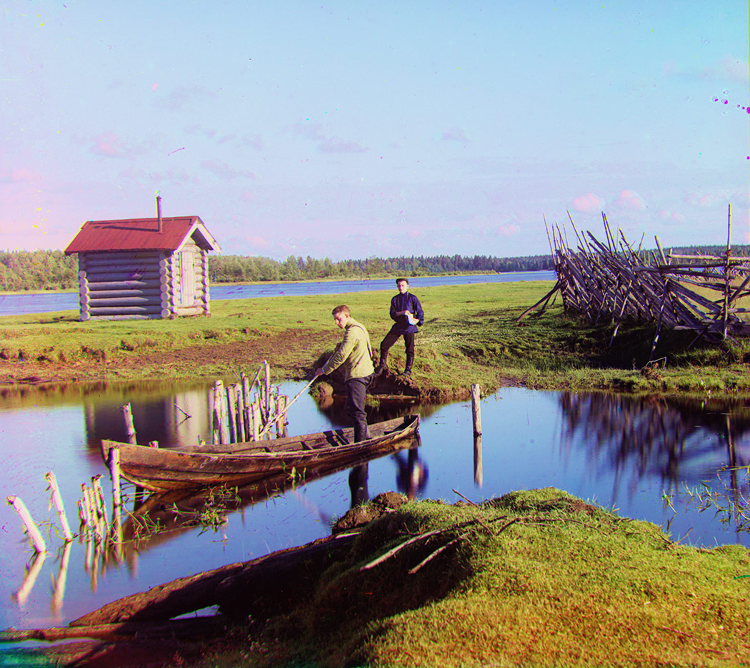
 Green Alignment Vector: [42 5]
Red Alignment Vector: [87 31] Cropping Rectangle: [218 244 3365 2938] Saturation Thresholds: [0.004, 0.765] Value Thresholds: [0.153 ,0.965] |
 Green Alignment Vector: [12 -5]
Red Alignment Vector: [133 -12] Cropping Rectangle: [205 259 3361 2995] Saturation Thresholds: [0.016, 0.694] Value Thresholds: [0.145, 0.957] |
 Green Alignment Vector: [-17 10]
Red Alignment Vector: [11 16] Cropping Rectangle: [187 134 3369 3012] Saturation Thresholds: [0.039, 0.867] Value Thresholds: [0.173, 0.922] |
 Green Alignment Vector: [71 39]
Red Alignment Vector: [148 63] Cropping Rectangle: [283 188 3306 2998] Saturation Thresholds: [0.016, 0.729] Value Thresholds: [0.184, 0.957] |
More Results
A few more examples that turned out nicely, taken from photographs of my own choosing:
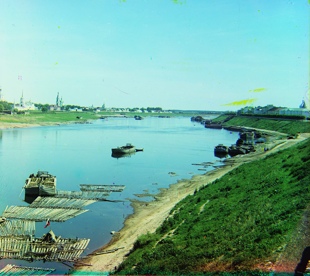 Green Alignment Vector: [39 15]
Red Alignment Vector: [91 33] Cropping Rectangle: [272 243 3311 2951] Saturation Thresholds: [0.102, 0.859] Value Thresholds: [0.122, 0.937] |
 Green Alignment Vector: [78 20]
Red Alignment Vector: [152 25] Cropping Rectangle: [201 189 3381 3000] Saturation Thresholds: [0.024, 0.855] Value Thresholds: [0.165, 0.953] |
 Green Alignment Vector: [57 21]
Red Alignment Vector: [138 38] Cropping Rectangle: [214 177 3310 2792] Saturation Thresholds: [0.020, 0.859] Value Thresholds: [0.078, 0.961] |
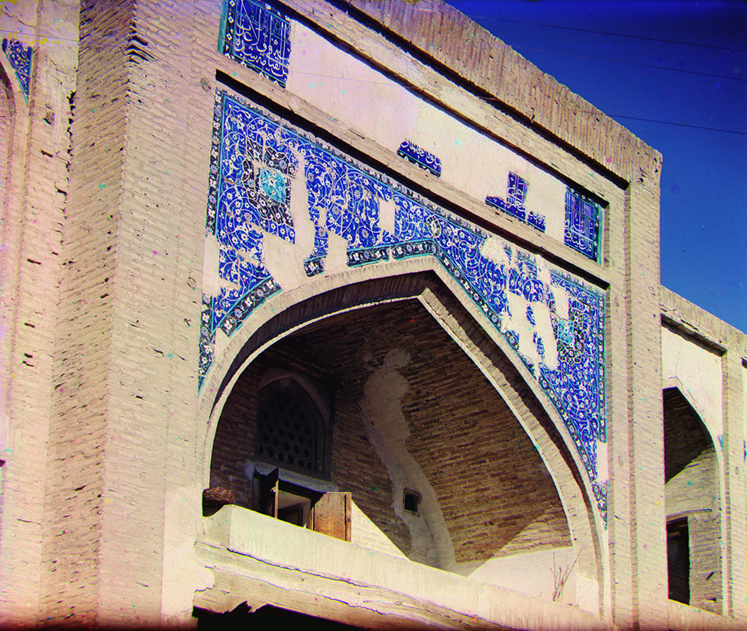
"Almost..."
It seems that the automated cropping algorithm is the least robust of the three, as it failed to suitably crop two of the assigned images. The likely explanation is that both plates have writing marked in the black border surrounding the image, tricking the border detection (which is based on brightness and color variation) into thinking the borders are a part of the image itself. Still, the alignment, color, and contrast procedures were successful (and the cropping is acceptable, if not quite aggressive enough).
 Green Alignment Vector: [24 20]
Red Alignment Vector: [72 33] Cropping Rectangle: [118 117 3439 3082] Saturation Thresholds: [0.078, 0.733] Value Thresholds: [0.169, 0.847] |
 Green Alignment Vector: [48 9]
Red Alignment Vector: [116 11] Cropping Rectangle: [215 182 3415 2941] Saturation Thresholds: [0.051, 0.871] Value Thresholds: [0.200, 0.953] |
Just For Fun...
Just for fun: what happens if we attempt to reproduce Prokudin-Gorskii's work with a modern digital camera? The camera already contains color filters (a Bayer grid, in most cases), so all that is really needed is a way to access the image sensor data before the camera adjusts it (i.e. RAW mode). Using a camera with RAW mode (here a Canon PowerShot G9) and the open-source DCRAW utility, it is possible to extract the sensor data in a way consistent with our use of Prokudin-Gorskii's plates. Specifically, it is possible to override any color space conversions, white balance adjustments, etc. and simply use the unmodified sensor data for R,G, and B. (This parallels our use of the Prokudin-Gorskii images because we lack specific information on the color properties of his filters, the sensitivity of his glass plate emulsion, etc.). The pertinent command line options for DCRAW are:
- -r 1 1 1 1: Custom white balance setting to leave the RGB values unchanged.
- -M: Ignore embedded color matrix information.
- -o 0: Do not perform any color space conversions.
- -W: Don't automatically brighten the image.
A simulated Prokudin-Gorskii "BGR" plate, and the output of the restoration code written for this project, are reproduced below:
 |

|
Green Alignment Vector: [0 0]
Red Alignment Vector: [0 0]
Cropping Rectangle: [466 75 3502 2949]
Saturation Thresholds: [0.000, 0.847]
Value Thresholds: [0.059, 1.000]
The result is mostly as expected: no offset is required for alignment, the cropping algorithm is too aggressive when there are actually no borders to be cropped, and the S and V channel ranges are expanded. However, the image is surprisingly green (and appears that way when rendered by Photoshop as well).
It turns out that the native output of the G9's sensor under daylight conditions requires significant white balance correction in order to produce a realistic color image. Normally, this correction would be performed either in the camera (when outputting JPEG) or by the RAW conversion utility but in this case it was deliberately disabled. My Prokudin-Gorskii image restoration code does not perform this correction because (as shown by the results above), most Prokudin-Gorskii images do not seem to require it.