In this section, we extend the analysis in
Section 3.5.1 to the general FB process. As in
Section 3.5.1, once the background process is approximated
by a Markov chain on a finite state space, it is straightforward to
reduce the FB process to a 1D Markov chain.
Hence, in this section, we limit our focus on approximating
the background process by a Markov chain on a finite state space;
for completeness, we formally describe the construction of the 1D Markov chain
using the approximated background process in Appendix 3.5.5.
We will see that, in general, a
collection of PH distributions is needed in the
approximate background process, ![]() , (e.g. recall Section 3.1.2) to capture
the dependency in the sequence of sojourn times in levels
, (e.g. recall Section 3.1.2) to capture
the dependency in the sequence of sojourn times in levels ![]() that
that ![]() has.
This is in contrast to the case when the background process is a
birth-and-death process, which required only a single PH distribution
in the approximate background process,
since the sojourn times in levels
has.
This is in contrast to the case when the background process is a
birth-and-death process, which required only a single PH distribution
in the approximate background process,
since the sojourn times in levels ![]() are i.i.d. in this case.
Below, we use
are i.i.d. in this case.
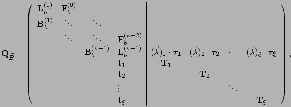
Below, we use ![]() to denote the generator matrix of
to denote the generator matrix of
![]() , and use
, and use
![]() ,
,
![]() ,
and
,
and
![]() to denote the submatrices of
to denote the submatrices of ![]() ,
following the convention introduced in Section 3.4
,
following the convention introduced in Section 3.4
We start by specifying the properties that ![]() should have.
Let
should have.
Let ![]() be the event that
the first state that we visit in level
be the event that
the first state that we visit in level ![]() is in phase
is in phase ![]() given that we transitioned from phase
given that we transitioned from phase
![]() in level
in level ![]() to any state in level
to any state in level ![]() .
(Notice that in the analysis of the M/PH/2 queue with two priority classes in Section 3.1,
each event
.
(Notice that in the analysis of the M/PH/2 queue with two priority classes in Section 3.1,
each event ![]() corresponds to the event that the phase of the job in service
immediately before a busy period starts is
corresponds to the event that the phase of the job in service
immediately before a busy period starts is ![]() and the phase of the job
in service immediately after the busy period is
and the phase of the job
in service immediately after the busy period is ![]() .)
We require that
.)
We require that
![]() has the following key properties:
has the following key properties:
To construct ![]() , we first analyze the probability
of event
, we first analyze the probability
of event ![]() and (the moments of) the distribution of the
sojourn time in levels
and (the moments of) the distribution of the
sojourn time in levels ![]() given event
given event ![]() (we denote this
distribution as
(we denote this
distribution as ![]() ) for each
) for each ![]() and
and ![]() .
(Notice that in the analysis of the M/PH/2 queue with two priority classes in Section 3.1,
.
(Notice that in the analysis of the M/PH/2 queue with two priority classes in Section 3.1,
![]() corresponds to the distribution of the busy period duration
given that the phase of the job in service
immediately before a busy period starts is
corresponds to the distribution of the busy period duration
given that the phase of the job in service
immediately before a busy period starts is ![]() and the phase of the job
in service immediately after the busy period is
and the phase of the job
in service immediately after the busy period is ![]() .)
Let
.)
Let ![]() be the number of phases in level
be the number of phases in level
![]() of
of ![]() (and
(and ![]() ). Then, there are
). Then, there are ![]() types of events
types of events ![]() .
.
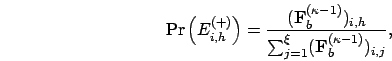
The probability of event ![]() is relatively easy to analyze.
Let
is relatively easy to analyze.
Let ![]() be a matrix of order
be a matrix of order ![]() whose
whose ![]() element is
the probability of event
element is
the probability of event ![]() .
Let
.
Let ![]() be the event that
be the event that
![]() transitions to state
transitions to state ![]() given that
the transition is from state
given that
the transition is from state ![]() to any state in level
to any state in level ![]() .
Also, let
.
Also, let ![]() be the event that
state
be the event that
state ![]() is the first state that
is the first state that ![]() hits in level
hits in level ![]() given that
given that
![]() starts in state
starts in state ![]() .
Then,
.
Then,
Next, we analyze the moments of ![]() .
Let
.
Let ![]() be a
matrix of order
be a
matrix of order ![]() whose
whose ![]() element is the
element is the ![]() -th moment
of
-th moment
of ![]() for
for ![]() .
Note that
.
Note that ![]() is a mixture of distributions of various conditional passage times
from level
is a mixture of distributions of various conditional passage times
from level ![]() to level
to level ![]() .
Specifically, let
.
Specifically, let
![]() be the time to go
from state
be the time to go
from state ![]() to state
to state ![]() .
Then, the distribution function of
.
Then, the distribution function of ![]() is given by
is given by
We are now ready to construct ![]() .
We use the moment matching algorithm developed in Chapter 2 to
approximate
.
We use the moment matching algorithm developed in Chapter 2 to
approximate ![]() by a PH distribution,
by a PH distribution,
![]() ,
matching the first three moments of
,
matching the first three moments of ![]() ,
,
![]() ,
for all
,
for all ![]() and
and ![]() .
Let
.
Let
![]() ,
where
,
where ![]() is a column vector with all elements 1 and has order
equal to the number of columns in
is a column vector with all elements 1 and has order
equal to the number of columns in
![]() .
.
Using ![]() and
and
![]() defined above,
the generator matrix of
defined above,
the generator matrix of ![]() is defined as
is defined as