Optimizing the Control of a Two-Link Pendulum
Tomasz Malisiewicz, Mark Palatucci, and Geoff Hollinger
Abstract
In this lab, we implemented LQR controllers and swing up optimization for a two-link pendulum. We examined three different actuator configurations: 1) The arm configuration uses a torque actuator at both the shoulder and elbow of the pendulum, 2) the acrobot uses only the elbow actuator, and 3) the whip uses only the shoulder actuator. We successfully designed an LQR controller for the arm by deriving the analytic system equations, and we designed LQR controllers for the other configurations by numerically differentiating the system dynamics. Finally, we designed an optimal swingup trajectory for the ARM by modifying CGA's dynamic programming implementation.
Analytical Derivation of LQR Controllers
To design LQR controllers for the two-link pendulum, we first derived the equations of motion using Lagrangian dynamics. The derivation of the A, B, Q, and R matrices for the LQR optimization is given below:
Running Matlab's lqrd function on these equations results in the following K matrix. These constants were able to hold the arm up indefinitely for any initial angle.
For the arm, the LQR controller was able to swing the arm up from a zero initial condition as shown in the following animation. The score of this swing up was 49.5027.

LQR controllers for the whip and acrobot were designed using the analytic derivation, but these controllers performed poorly. To improve the performance of these controllers, we numerically differentiated the system constants as described in the next section.
The code for this section is given in the folder armAnalytical in the tarball. The A, B, K, Q, and R files give the respective matrices, and the lqrArmAnalytical.m file gives the Matlab code for running lqrd on the system.
Derivation of LQR Controllers Using Numerical Differentiation
We also computed the constants using a numerical method. We used the program
"linearize-dynamics-2-link" (located in hw2solution/dynamics/linearize-dynamics-2-link)
provided by CGA to simulate the dynamics of the system. We found the A and B
matrices of the whole ARM system to be:

We then computed Q and R matrices from the cost function that CGA provided.

Taking our A,B,Q,R matrics we computed a LQR controller in Matlab. Since we already
discretized the system, we used the "dlqr" command instead of the "lqrd" command. We found
the constants for the ARM were:

Computing the constants for WHIP and ACROBOT was very similar. The A matrix doesn't change since
we're not changing the dynamics of the system - just the action dimension. After much fiddling, we discovered
that the easiest way to compute a new B is to simply 'zero out' the appropriate column in the B matrix we found previously.
For the WHIP, we want to remove all the torque from the elbow servo. We can do this by zero'ing the 2nd column
our B matrix.

We then plugged this back into "dlqr" using the same A, Q, R as before. We found the constants for the WHIP to be:

We did the same thing for the ACROBOT and found B:

and the constants for the ACROBOT were:

In order to use these constants to test the ARM, WHIP, and ACROBOT we modified the "ass2kdc" program that CGA provided. (See
hw2solution/ass2kdc-numeric-k.cpp). This program takes an initial state as usual. It was modified to read a file "K" that
provides the above constants. We computed the torques by modifying the simLoop function with the following code:

Results
ARM: We were easily able to balance the ARM at the top. Further, we tried several initial states and found that the ARM will always stabilize at the top.
WHIP: We found that we could balance the WHIP at the top. The system could balance even if the starting angle was 3.01 rads. At 3.0 rads, the system will collapse.
ACROBOT: We found that we could balance the ACROBOT the top. The system was much more fragile than the WHIP though - with an initial angle at 3.13 rads we could still balance,
but at 3.129 rads the system would collapse.
Code
See "hw2solution/ass2kdc-numeric-k". Copy the constants for whichever system you want to test to "K". E.g. "cp K-whip-good K". Then run
ass2kdc-numeric-k with the initial state. E.g. "ass2kdc-numeric-k 3.13 0 0 0"
Keep Your Friends Close and Your Markov Blankets Closer
Our initial attempt at the dynamic programming solution to part2 consisted of modifying our dynamic programming implementation from assignment one. Rather than performing a sweep of the entire state-space at each iteration, we implemented a dijkstra-like algorithm (we tried following the Obtaining Dijkstra-like algorithms section of LaValle's book). However, since obtaining the backprojection at a given point in state space is not easy we used an approximation to the true Front such that the true frontier is a proper subset of the approximate Front. For the approximate front, we tried using a markov blanket of order K (all states surrounding the current state inside a rectangular region of width K, where K is some integer). The basic idea was to reduce the amount of computation in each value iteration; however, this markov blanket of order K concept proved to be not as great as expected. In essence, neighbors on the grid of states are not necessarily neighbors according to the dynamics of the system and in order to make sure that the approximate Front contains the true frontier as a proper subset, K had to be set to a very large number -- this made the algorithm quite inefficient. From our experience, K had to be set so large that it was more expensive to maintain the dead/alive/unvisited states than performing sweeps over the entire state space at each iteration.
We decided to perform full sweeps over state space at each stage of value iteration, and thus chose to modify CGA's dynamic programming implementation.
When modifying CGA's code, we had to implement multilinear interpolation and use the LQR results from part one (numeric differentiation). The following results were generated using a discrete grid of size 31 x 31 x 31 x 31 .
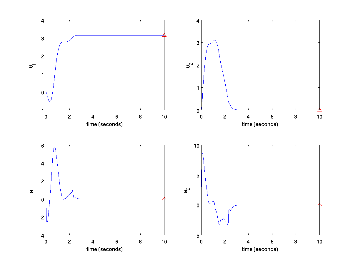
The above figure shows the state of the ARM as a function of time. The goal state is represented as a red triangle on the right side of each plot. One can clearly see that we reached the goal configuration in well under 10 seconds.
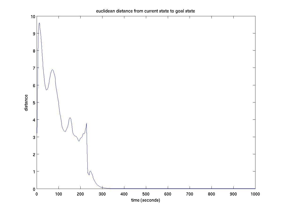
The above figure shows the euclidean distance from the current state to the goal state as a function of time. Even though the euclidean distance over state variables is not a meaningful quantity (using different units will change the distance), it is interesting to see that the distance to goal is not a monotonically decreasing function. This shows how dynamic programming obtains an optimal solution -- a solution that does not necessarily bring us closer to the goal greedily at each time step.
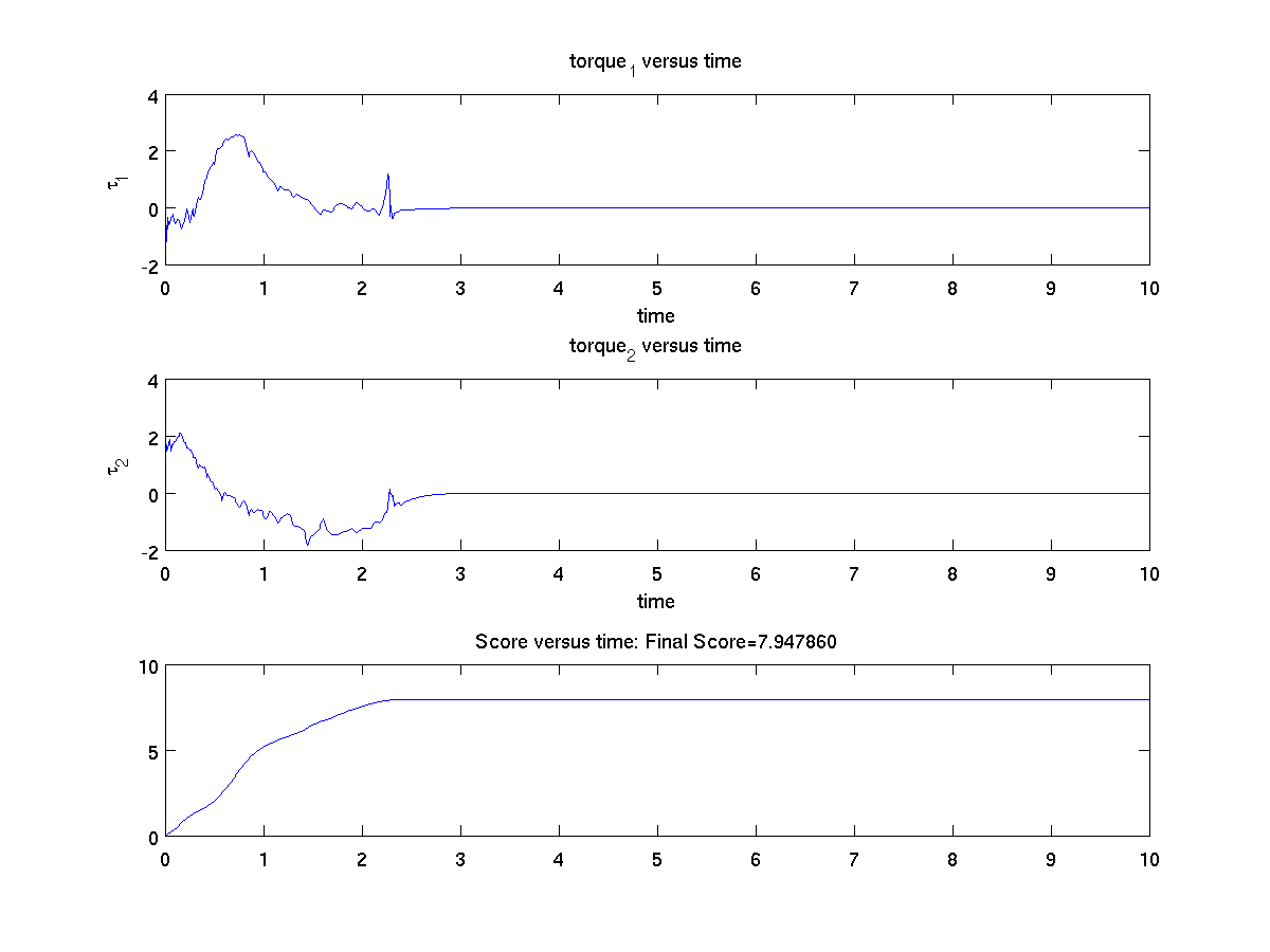
This figure displays the policy as a function time. In this case, the policy is two dimensional -- one torque for each of the two joints. We have also plotted the score as a function of time.
The final score for 10 seconds of the ARM was 7.95.
The code for part two of this assignment can be found in hw2solution/part2/. After running make, one must run do the following to produce the trajectory:
./make-model
./dp
./use-policy
At this point, one can run the show_traj matlab script to display the trajectories graphically.
Code
The link below gives the code for this lab. To run, unzip the directory, type make, and run ass2kdc.
References
The web page for this assignment can be found below:
Obtaining Dijkstra-like algorithms section of LaValle's book